Mean decomposition of a variable by group(s)

This function decomposes a variable in a long data set by grouping factors, such as by ID. If multiple grouping factors are listed, the decomposition is in order from left to right. Residuals from the lowest level are returned.

Usage

meanDecompose(formula, data)

Arguments

formula

A formula of the variables to be used in the analysis. Should have the form: variable ~ groupingfactors.

data

A data table or data frame containing the variables used in the formula. This is a required argument.

Value

A list of data tables with the means or residuals

Examples

meanDecompose(mpg ~ vs, data = mtcars)
#> $`mpg by vs`
#>       vs        X
#>    <num>    <num>
#> 1:     0 16.61667
#> 2:     1 24.55714
#> 
#> $`mpg by residual`
#>              X
#>          <num>
#>  1:  4.3833333
#>  2:  4.3833333
#>  3: -1.7571429
#>  4: -3.1571429
#>  5:  2.0833333
#>  6: -6.4571429
#>  7: -2.3166667
#>  8: -0.1571429
#>  9: -1.7571429
#> 10: -5.3571429
#> 11: -6.7571429
#> 12: -0.2166667
#> 13:  0.6833333
#> 14: -1.4166667
#> 15: -6.2166667
#> 16: -6.2166667
#> 17: -1.9166667
#> 18:  7.8428571
#> 19:  5.8428571
#> 20:  9.3428571
#> 21: -3.0571429
#> 22: -1.1166667
#> 23: -1.4166667
#> 24: -3.3166667
#> 25:  2.5833333
#> 26:  2.7428571
#> 27:  9.3833333
#> 28:  5.8428571
#> 29: -0.8166667
#> 30:  3.0833333
#> 31: -1.6166667
#> 32: -3.1571429
#>              X
#> 
meanDecompose(mpg ~ vs + cyl, data = mtcars)
#> $`mpg by vs`
#>       vs        X
#>    <num>    <num>
#> 1:     0 16.61667
#> 2:     1 24.55714
#> 
#> $`mpg by vs & cyl`
#>       vs   cyl         X
#>    <num> <num>     <num>
#> 1:     0     6  3.950000
#> 2:     1     4  2.172857
#> 3:     1     6 -5.432143
#> 4:     0     8 -1.516667
#> 5:     0     4  9.383333
#> 
#> $`mpg by residual`
#>              X
#>          <num>
#>  1:  0.4333333
#>  2:  0.4333333
#>  3: -3.9300000
#>  4:  2.2750000
#>  5:  3.6000000
#>  6: -1.0250000
#>  7: -0.8000000
#>  8: -2.3300000
#>  9: -3.9300000
#> 10:  0.0750000
#> 11: -1.3250000
#> 12:  1.3000000
#> 13:  2.2000000
#> 14:  0.1000000
#> 15: -4.7000000
#> 16: -4.7000000
#> 17: -0.4000000
#> 18:  5.6700000
#> 19:  3.6700000
#> 20:  7.1700000
#> 21: -5.2300000
#> 22:  0.4000000
#> 23:  0.1000000
#> 24: -1.8000000
#> 25:  4.1000000
#> 26:  0.5700000
#> 27:  0.0000000
#> 28:  3.6700000
#> 29:  0.7000000
#> 30: -0.8666667
#> 31: -0.1000000
#> 32: -5.3300000
#>              X
#> 

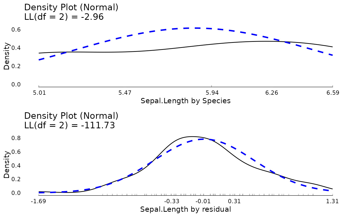
## Example plotting the results
tmp <- meanDecompose(Sepal.Length ~ Species, data = iris)
do.call(ggpubr::ggarrange, c(lapply(names(tmp), function(x) {
  plot(JWileymisc::testDistribution(tmp[[x]]$X), plot = FALSE, varlab = x)$Density
}), ncol = 1))


rm(tmp)